Activity 17: Photometric Stereo

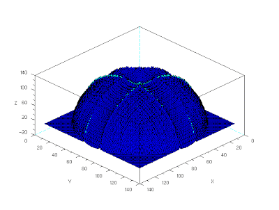
Photometric stereo uses light intensity from different light sources to infer the shape of a three-dimensional surface. For this activity we used four images of a sphere illuminated with four light sources positioned at different locations. For each source, the corresponding images are the following

Figure 1. Images

The reconstruction is shown below

Figure 2. Reconstruction.

The reconstruction is imperfect as shown in figure 2. However, to some extent the 3D features of our object has been reconstructed.

For this activity, I'll give myself a 9 because my code uses lots of for loops.

Activity 16: Neural Network

This activity uses the same training and test sets as with the previous activities. The algorithm for the neural network requires us to "label" the classes that will be used for the training. These labels will then be used to classify the test set. If a test object gives an array similar to the "label" of a certain class, it is assigned to that class. Note that we used five nodes for the output layer. This was done so that there will be a high difference between classes.

Figure 1. Training set labels.

The implementation of the neural network is separated in two. One, with a learning rate of 0.1 while the other has a learning rate of 2.5. The results are shown below (click for a larger image)

Figure 2. Summary of results. Left: Learning rate = 0.1. Right: Learning rate = 2.5.

Cells with red shading indicates wrong classification. These false results are observed only with a neural network with low learning rate. For 2.5 learning rate, the classification is 100% accurate. Also, compared to the previous methods, neural network shows a sharp distinction between classes. The values shown in figure 2 demonstrate this.


For this activity, I'll give myself a 9 for completing the activity and for the effort of figuring out how to implement a five node output layer neural network.

Activity 15: Probabilistic Classification

This objective of this activity is similar to that of activity 14. Here we will be using the linear discriminant analysis formula given by

Where µi is mean of the features of class i, x is the matrix of the features of object k, C is the covariance matrix. The object k is assigned to class i that has maximum fi [1]

Here we used the same training set and test set as with activity 14. The result is shown below.

Table 1. Summary of result.

Again, the result shows 100% accuracy. The two coins are still close as with activity 14.

For this activity I'll give myself 10 for completing the activity.

Reference:

[1] Teknomo, Kardi. Discriminant Analysis Tutorial. http://people.revoledu.com/kardi/ tutorial/LDA/

Activity 14: Pattern Recognition

For this activity, we tried to simulate the human brain’s capacity to differentiate objects. We extracted features of different objects that can be compared (e.g. RGB components, area, eccentricity, etc). If a test object has features that is close to the features of a certain class, we assign it to that class.

First a training set is prepared to have a basis of comparison. The test objects are the following

Figure 1. Training set.

The feature of each class is plotted (i.e. RG components, eccentricity).

Figure 2. Plot of the features of the training set.

To determine which class a test object belongs, we used the Euclidean distance

Where dj represents the distance to class j, x is a matrix containing the features of the test object (the superscript T means transpose) and mj is the mean of the features of the class j. The test object is assigned to the class that gives the largest d. The results are as follow

Table 1. Summary of results.

The result shows 100% accuracy of the method for the chosen test objects. However it should be noted the closeness of values for the coin test objects indicating that the method and/or the features chosen is insufficient to create a sharp distinction between very similar objects.

For this activity, I'll give myself a 10 for completing it and for having satisfactory results.

Activity 13: Correcting Geometric Distortions

Distortion is an example of monochromatic aberrations. Distortion arises because different areas of the lens have different focal length and different magnifications. There are two types of distortion positive or pincushion distortion and negative or barrel distortion. Ideally, a thin lens will have no distortion. [1]

Figure 1. Left: Barrel distortion. Right:Pincushion distortion. If there is no distortion, the above images will be regularly spaced grids.

For this activity, we are tasked to correct a distorted image by first assuming that the distorted image is just a linear transform of the ideal image and vice versa.

Figure 2. Coordinate transformation.

The transformation functions are assumed to be bilinear functions of the form

where x and y in the LHS are the pixel coordinates in the distorted image and the x and y in the RHS are for the ideal image. After finding the coordinate transform, we look for the grayvalue at the ideal image pixel locations using a bilinear interpolation.

For my distorted images, I used the ones below (Click for a larger view.)

Figure 3. Distorted images.

The results are the following. (Click for a larger view.)

Figure 4. Corrected images.

Then results show that the method is sufficient to correct distortion of small images.

For this activity, I'll give myself a 10 for satisfactory result. Note that the reconstructed image does not require anymore a second bilinear interpolation because no null pixels are found.

Reference
[1] E. Hecht (2002). Optics 4th edition. Addison Wesley , CA.