Activity 10: Preprocessing Text

In this activity, we are asked to extract information from a scanned document (figure 1) specifically handwriting. This activity is the integration of the techniques learned from the previous activities. The first task at hand is to clean the image by removing the horizontal and vertical lines present. Here we used filtering just like in activity 7. For this part only a portion of the image is used.

Figure 1. Left: The scanned document. Right: Cropped document.

The image is binarized and inverted (i.e. high becomes low) since we are interested in the text hence it should have a value of 1 (i.e. it should be white).

Figure 2. Top left: Binarized image. Top right: Its FFT. Bottom left: The filter which is binarized before multiplying with the FFT. Bottom right: The filtered image.

For further cleaning of unwanted white dots, morphological operations are also used from Activity 8 and 9.

Figure 3. Left: Binarized image of the filtered image. Right: Image after opening operation

After cleaning, thinning is applied to make the text one pixel thick.

Figure 4. Image after thinning operation.

The text in the final image is not recognizable indicating that the cleaning procedure is insufficient.

Finally, correlation is also used to find occurances of the the word "DESCRIPTION" utilizing the technique in activity 5.

Figure 5. Locations of the word "DESCRIPTION". (Click to enlarge.)

What's annoying...
Scilab crashes in Windows Vista when mogrify is used.

For this activity, I'll give myself a 10 because I was able to use the techniques in the previous activities although I'm still not good at filtering. Finding the right filter is a hard task.

Activity 12: Color Image Segmentation

For this activity, we separated a particular color in an image. If a color of an object in an image is uniform (i.e. no shading variations), it is relatively much easier to separate that particular object. However, this becomes difficult when dealing images of three dimensional objects because of shading variations. To do this, we must indicate a "range" of colors that are present in an object (or more properly called as region of interest). To methods are presented here: parametric and non-parametric. Parametric approach uses a function to specify the probability of a color to be present in the ROI. The parameters of the function are computed from a patch of the ROI. Non-parametric involves counting of the colors present in the ROI patch and the histogram of which is taken as the probability distribution. The quality of segmentation depends on the size of the bins used in the histogram. The results are as follows

Figure 1. Left: Original image. Middle: Parametric segmentation showing only orange objects. Right: Parametric segmentation showing only red objects.



Figure 2. Non-parametric segmentation with varying bin sizes 10, 32, 64 from left to right. Top row: Segmentation for orange objects. Bottom row: Segmentation for red objects.

From figure 1 and 2, it can be noticed that the segmentation is not perfect. This is because of the limited size of the patch that used and also some of the objects in the image has some of the colors of the ROI.

For this activity, I'll give myself a 9. I have to admit that this was done in a hurry. I still have lots of images but for reason of time conservation I opted to post just a few.

Activity 11: Color Image Processing

Improperly white balanced images will result in incorrectly represented colors. Modern cameras has auto-white balance capability to ensure correct representation and other presets for different lighting conditions. For this activity we captured images by using the presets (e.g. daylight, cloudy, fluorescent, incandescent) and perform white balancing algorithm to correct the captured images.

The algorithm that will be used are the white patch algorithm and the gray world algorithm. The white patch algorithm uses the average RGB values of a white object in the image as balancing constants. While the gray world algorithm averages the RGB of the whole image and uses it as balancing constant. Below are images taken outdoors and indoors under different white balancing presets in the camera. The camera used is a cellphone camera (i.e. Sony Ericsson K550i with 2MP camera)

Figure 1. Outdoor images. First column: Original image. Second column: Balanced using white patch algorithm. Third column: Balanced using gray world algorithm. The rows represent the white balancing preset used. First row: Daylight. Second row: Cloudy. Third row: Fluorescent. Fourth row: Incandescent.




Figure 2. Indoor images. First column: Original image. Second column: Balanced using white patch algorithm. Third column: Balanced using gray world algorithm. The rows represent the white balancing preset used. First row: Daylight. Second row: Cloudy. Third row: Fluorescent. Fourth row: Incandescent.

From the two sets of images, indoor and outdoor, the white patch algorithm produces better color representation than the gray world algorithm. In white patch algorithm, white objects indeed appears white. White objects serve as basis for the white balancing. Gray algorithm highly depends on the dominant color in the image. More clipping is also observed in gray world algorithm. Both algorithms were also tested with subjects that has a dominant color which in this case is red

Figure 3. Indoor incorrectly white balanced images with red as dominant. First column: Original image. Second column: Balanced using white patch algorithm. Third column: Balanced using gray world algorithm. The rows represent the white balancing preset used. First row: Incandescent. Second row: Daylight. Third row: Cloudy.

Figure 3 shows that white patch algorithm still produces more decent result. The gray world algorithm produces images with a shade different from the dominant. For example, in the first row of figure 3, the result of the gray world algorithm has a shade of blue. For daylight and cloudy presets, the shade is yellow.

For this activity, I'll give myself a 10 for completing the activity and for the effort to finish this. This blog is posted using only a cellphone with GPRS connected to a laptop.

Activity 9: Binary Operation

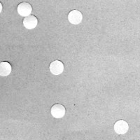
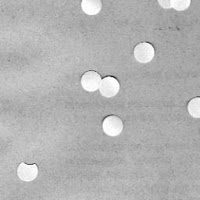
For this activity, we are given an image consisting of circular objects which may be thought of as cells. The objective is to find the average area of the cell. One approach is to count it manually. This is feasible for small image but definitely a problem for real world data processing. The best way is to program it, however one problem of this approach is that binarized image may not be clean. The presence of those tiny white dots may lead to incorrect area estimation.

Figure 1. Image to be processed.

To solve this issue, I used the morphological operation called opening with a small circle (with radius less than the radius of the cells) as structuring element. This is just erosion followed by dilation. The figure below shows how opening and its counterpart closing works. (Image taken from http://ikpe1101.ikp.kfa-juelich.de/briefbook_data_analysis/node178.html)

Figure 2. Demonstration of the opening and closing operation.

Below are the sub-images of figure 1 each having a dimension 256x256.

Figure 3. Sub-images from figure 1.

The sub-images in figure 3 are binarized so that opening can be applied. After bwlabel was used to tag each blob. Finally, the area of each blob are tallied.

Figure 4. Sub-images after labeling. For visual clarity, jet colormap is used.

The result of the histogram is as follows.

Figure 5. Histogram of area of the blobs.

Upon removal of the outliers (i.e. area>600 and area<300), a value of 487 for the mean area was computed with standard deviation of 59. The histogram in figure 5 corresponds to this result.

For this activity, I'll give myself a 10 for completing the activity and producing satisfactory result.