Activity 4: Enhancement by Histogram Manipulation

For this activity, poor contrast images are improved by re-mapping of pixel values. The whole method is schematically show below

Figure 1. Schematic diagram showing the cumulative frequency distribution (CDF) of the original image and the desired CDF.

Referring to figure 1, for each pixel value of the original image get its cumulative frequency (i.e. value at the y-axis; step 1 & 2). See if there is a corresponding value in the desired CDF (step 3). If there is, check its corresponding pixel value (step 4) and use this to replace the pixel value in the original image.

Here are my results. (Click on the figure to enlarge.)

Figure 2. Top: Original image. Middle: PDF of the original image. Bottom: The corresponding CDF.

Figure 3. Top: Original image. Middle: PDF of the original image. Bottom: The corresponding CDF.

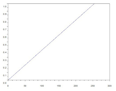
For contrast enhancement, I used a linear CDF and a logarithmic CDF. Below are the graphs of their CDFs

.

Figure 4. Left: Linear CDF. Right: Logarithmic CDF.

The reconstructed images with their corresponding CDFs are as follows.

Figure 5. Upper left: Reconstructed image using linear CDF. Upper right. The corresponding CDF. Lower left: Reconstructed image using logarithmic CDF. Lower right: The corresponding CDF.

Figure 6. Upper left: Reconstructed image using linear CDF. Upper right. The corresponding CDF. Lower left: Reconstructed image using logarithmic CDF. Lower right: The corresponding CDF.

The CDFs of the reconstructed images follow the general shapes of the desired CDFs. In the logarithmic CDF, there is preference to lower pixel values hence the reconstructed image appears darker.

Below is the code that I've used.

chdir('C:\Users\Mark Jayson\Documents\Physics\APhysics 186\Act 4');

I=imread('test04.png');
I=im2gray(I);

//pdf of original image
m=tabul(I, 'i');
total=256*256;
datapdf=[0:255]';
zer=zeros(256,1);
datapdf=cat(2,datapdf,zer);

for i=1:length(m(:,1))
init=int(m(i,1))+1;
datapdf(init,1)=m(i,1);
datapdf(init,2)=m(i,2)/total;
end

plot(datapdf(:,1),datapdf(:,2));
xlabel('pixels');


//cdf of original image
m2=cumsum(datapdf(:,2));
datacdf=cat(2,datapdf(:,1),m2);
scf(1);
plot(datacdf(:,1),datacdf(:,2));
xlabel('pixels');

//cdf2: linear cdf
datacdf2=[0:255]';
temp=[0:255]'/255;
datacdf2=cat(2,datacdf2,temp);
scf(2);
plot(datacdf2(:,1),datacdf2(:,2))
xlabel('pixels');

//cdf4: logarithmic cdf
hmneye=log([1:256])';
pixel=[0:255]';
datacdf4=cat(2,pixel,hmneye/max(hmneye));
scf(3);
plot(datacdf4(:,1),datacdf4(:,2));

//Note: comment out cdf2 or cdf4 if you wish to use logarithmic or linear cdf respectively

//mapping
temp=zeros(256,256);
temp1=floor(datacdf(:,2)*255);
temp2=floor(datacdf4(:,2)*255);

for i=1:length(datacdf(:,2))
ii=find(temp2==temp1(i));
temp=temp+datacdf4(ii(1),1)*(I==datacdf(i,1));
end

//cdf recon
m=tabul(temp, 'i');
total=256*256;
pdf=[0:255]';
zer=zeros(256,1);
pdf=cat(2,pdf,zer);

for i=1:length(m(:,1))
init=int(m(i,1))+1;
pdf(init,1)=m(i,1);
pdf(init,2)=m(i,2)/total;
end

m2=cumsum(pdf(:,2));
cdf=cat(2,pdf(:,1),m2);
scf(4);
plot(cdf(:,1),cdf(:,2)); //cdf of reconstructed image
xlabel('pixels');

scf(5); imshow(I/255); //original image
scf(6); imshow(temp/255); //reconstructed image


For this activity I'll give myself a 10 because I was able to do the activity well and I've discovered a function in scilab called tabul() which tabulates pixel values and their corresponding frequencies (although there is a more efficient way of doing this). This activity is fun! ^_^